import numpy as np
import matplotlib.pyplot as plt
import pandas as pd
import gro_exp
Example Notebook for pyDB
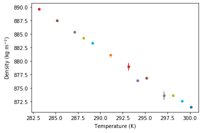
Read the density data from two components from a DDB Data Excel File over a specified temperature area for a pressure of 1 bar
# Set the tempature area
temp_vec = np.linspace(280.15,300.15,21)

# Read the data with the following function
data, prop_dict = gro_exp.ddb.read_exp_temp_vec("benzene_exp_density.xls", temp_vec, "DEN",
                        press=101325.000,tol_p=10000, p_nan=False, is_plot=True, is_display=False)
The data dictionary contains the Mean properties, standard deviation and number of data points at the specified temperatures. The prop_dict dictonary contains the data points which are used to calculate the mean values at the specified temperature. In the following cell shows some content for these dictonarys
# Define the temperature which you would like consider
temp = 288.15

# Data frames
df_mean = pd.DataFrame(data)
display(df_mean)
| Temperature (K) | DEN (kg/m3) | STD (kg/m3) | Number of data points | References | |
|---|---|---|---|---|---|
| 0 | 280.15 | NaN | NaN | NaN | [] |
| 1 | 281.15 | NaN | NaN | NaN | [] |
| 2 | 282.15 | NaN | NaN | NaN | [] |
| 3 | 283.15 | 889.606250 | 0.208877 | 12.0 | [Sun T.F., Schouten J.A., Trappeniers N.J., Bi... |
| 4 | 284.15 | NaN | NaN | NaN | [] |
| 5 | 285.15 | 887.500000 | 0.000000 | 1.0 | [Wang F., Evangelista R.F., Threatt T.J., Tava... |
| 6 | 286.15 | NaN | NaN | NaN | [] |
| 7 | 287.15 | 885.400000 | 0.000000 | 1.0 | [Wang F., Evangelista R.F., Threatt T.J., Tava... |
| 8 | 288.15 | 884.275056 | 0.154745 | 18.0 | [Nowak J., Malecki J., Thiebaut J.-M., Rivail ... |
| 9 | 289.15 | 883.340000 | 0.140000 | 2.0 | [Meyer J., Mylius B., Z.Phys.Chem.(Leipzig), 9... |
| 10 | 290.15 | NaN | NaN | NaN | [] |
| 11 | 291.15 | 881.100000 | 0.000000 | 1.0 | [Wang F., Evangelista R.F., Threatt T.J., Tava... |
| 12 | 292.15 | NaN | NaN | NaN | [] |
| 13 | 293.15 | 878.951217 | 0.657108 | 69.0 | [Wang F., Evangelista R.F., Threatt T.J., Tava... |
| 14 | 294.15 | 876.400000 | 0.000000 | 1.0 | [Golubev I.F., Frolova M.G., Trudy Gos.NIPI In... |
| 15 | 295.15 | 876.900000 | 0.000000 | 1.0 | [Wang F., Evangelista R.F., Threatt T.J., Tava... |
| 16 | 296.15 | NaN | NaN | NaN | [] |
| 17 | 297.15 | 873.600000 | 0.778888 | 3.0 | [Hayworth K.E., Lenoir J.M., Hipkin H.G., J.Ch... |
| 18 | 298.15 | 873.548792 | 0.825668 | 197.0 | [Nowak J., Malecki J., Thiebaut J.-M., Rivail ... |
| 19 | 299.15 | 872.600000 | 0.000000 | 1.0 | [Wang F., Evangelista R.F., Threatt T.J., Tava... |
| 20 | 300.15 | 871.500000 | 0.000000 | 1.0 | [Singh S., Sivanarayana K., Kushwaha R., Praka... |
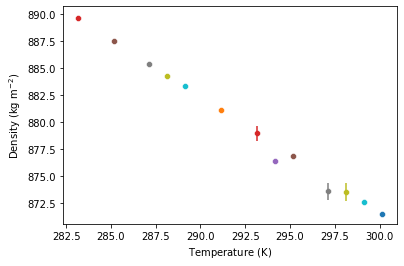
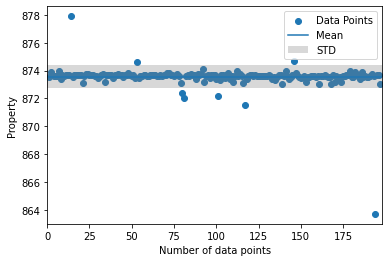
It is possible to plot the data points at a temperature to see the outliers
# Plot data for a specified temperature
temp=298.15
temp_off = gro_exp.ddb.plot_data(prop_dict,temp)
| Mean | STD | Number of data points | |
|---|---|---|---|
| 298.15 | 873.548792 | 0.825668 | 197 |
If you specified the outliers you can drop these and calculate a new data dictonary
# Drop outliers for the considered temperature
df_mean = pd.DataFrame(data)
data = gro_exp.ddb.drop_outliers(data,prop_dict,temp, [872,876])
display(df_mean)
| Temperature (K) | DEN (kg/m3) | STD (kg/m3) | Number of data points | References | |
|---|---|---|---|---|---|
| 0 | 280.15 | NaN | NaN | NaN | [] |
| 1 | 281.15 | NaN | NaN | NaN | [] |
| 2 | 282.15 | NaN | NaN | NaN | [] |
| 3 | 283.15 | 889.606250 | 0.208877 | 12.0 | [Sun T.F., Schouten J.A., Trappeniers N.J., Bi... |
| 4 | 284.15 | NaN | NaN | NaN | [] |
| 5 | 285.15 | 887.500000 | 0.000000 | 1.0 | [Wang F., Evangelista R.F., Threatt T.J., Tava... |
| 6 | 286.15 | NaN | NaN | NaN | [] |
| 7 | 287.15 | 885.400000 | 0.000000 | 1.0 | [Wang F., Evangelista R.F., Threatt T.J., Tava... |
| 8 | 288.15 | 884.275056 | 0.154745 | 18.0 | [Nowak J., Malecki J., Thiebaut J.-M., Rivail ... |
| 9 | 289.15 | 883.340000 | 0.140000 | 2.0 | [Meyer J., Mylius B., Z.Phys.Chem.(Leipzig), 9... |
| 10 | 290.15 | NaN | NaN | NaN | [] |
| 11 | 291.15 | 881.100000 | 0.000000 | 1.0 | [Wang F., Evangelista R.F., Threatt T.J., Tava... |
| 12 | 292.15 | NaN | NaN | NaN | [] |
| 13 | 293.15 | 878.951217 | 0.657108 | 69.0 | [Wang F., Evangelista R.F., Threatt T.J., Tava... |
| 14 | 294.15 | 876.400000 | 0.000000 | 1.0 | [Golubev I.F., Frolova M.G., Trudy Gos.NIPI In... |
| 15 | 295.15 | 876.900000 | 0.000000 | 1.0 | [Wang F., Evangelista R.F., Threatt T.J., Tava... |
| 16 | 296.15 | NaN | NaN | NaN | [] |
| 17 | 297.15 | 873.600000 | 0.778888 | 3.0 | [Hayworth K.E., Lenoir J.M., Hipkin H.G., J.Ch... |
| 18 | 298.15 | 873.548792 | 0.825668 | 197.0 | [Nowak J., Malecki J., Thiebaut J.-M., Rivail ... |
| 19 | 299.15 | 872.600000 | 0.000000 | 1.0 | [Wang F., Evangelista R.F., Threatt T.J., Tava... |
| 20 | 300.15 | 871.500000 | 0.000000 | 1.0 | [Singh S., Sivanarayana K., Kushwaha R., Praka... |
Now you can plot and display the new mean values after the adjustment
gro_exp.ddb.plot_means(data)
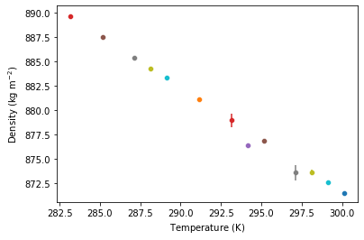
After all you can save the data in a obj file and reload at and plot it again
gro_exp.utils.save_data("test.obj",data)
data = gro_exp.utils.load_data("test.obj")
gro_exp.ddb.plot_means(data)